Let's discuss Mathematics

[Kyriakos]

@Samson , about the +- presentation, another thought of how it can be presented using not just the real number line but distance (absolute value). So Xo is used as a pivot point to max/min x, which turns it (in this world) into an analogue of 0. For the special case, Xo is 0. I included also one use within secondary education math. Other uses include limits (by just having an inequality instead of an equality).

 

[Kyriakos]

A question. The following is my proof that if you have two equations of the form:
ax^2+bx+c
cx^2+bx+a
with the coefficients having the same value (c,a,b) and just c and a changing positions,
also with c(a) not zero

then it follows (a) that of their two roots -as c(a) is not zero, there are two roots and none is zero-, one root of the first will be the reciprocal of one root of the second
and also (b) that actually both of their roots will be reciprocals of the other roots.

I wish to ask:
1) is this true? (that always both roots of the first will have a reciprocal in roots of the second)
2) can you think of a different way to prove this? (eg with identities to do with b and the root of the discriminant)
3) I suspect that the reciprocal is always one with altered position in regards to -b/coefficient of the stable term being added or subtracted from the square root of the discriminant - eg if x1=(-b+sqrootD)/2a, it will always be the reciprocal of x2'=(-b-sqrootD)/2c. Is this true?

Here are my solutions:

Thanks for any help Eg @a pen-dragon

 

[a pen-dragon]

This is indeed true and there is an easier (and more general) proof, providing a similar statement for any polynomial:

We want to solve a*x²+b*x+c=0. (Or the roots of an arbitrary polynomial)
Let r be the reciprocal of x. Then x=1/r and we obtain:
a*(1/r)²+b*(1/r)+c=0
If we multiply this by r² we get our final result:
c*r²+b*r+a=0

The condition that a and c must not be equal to zero emerges from demanding r to be finite and non-zero. a or c equal to zero will always produce a root at zero.

More generally this procedure will always reverse the order of the coefficients.


Concerning 3), this is indeed true, as can easily be checked by multiplying the standard solution of the roots. Note the order of the signs in the first terms is exchanged. Both cases result in the same.
(-b+-\sqrt(b²-4ac))/(2a)*(-b-+\sqrt(b²-4ac))/(2c) = (b²-(b²-4ac))/4ac = 1

 

[Kyriakos]

This is indeed true and there is an easier (and more general) proof, providing a similar statement for any polynomial:

We want to solve a*x²+b*x+c=0. (Or the roots of an arbitrary polynomial)
Let r be the reciprocal of x. Then x=1/r and we obtain:
a*(1/r)²+b*(1/r)+c=0
If we multiply this by r² we get our final result:
c*r²+b*r+a=0

The condition that a and c must not be equal to zero emerges from demanding r to be finite and non-zero. a or c equal to zero will always produce a root at zero.

More generally this procedure will always reverse the order of the coefficients.


Concerning 3), this is indeed true, as can easily be checked by multiplying the standard solution of the roots. Note the order of the signs in the first terms is exchanged. Both cases result in the same.
(-b+-\sqrt(b²-4ac))/(2a)*(-b-+\sqrt(b²-4ac))/(2c) = (b²-(b²-4ac))/4ac = 1

Thanks. For some bizarre reason I didn't bother with the direct multiplication to find a proof for question 3
And yes, the proof for question1 is certainly more condensed and alludes to more general use too - although I constructed my own meaning to use it for question3...

 

[Samson]

I am trying to get a simple overview of the geometry of gravity waves. The best explaination I found is Slides 7 - 18 of the presentation below, but I got a bit lost at the last few stages with gauge conditions and polarization tensors and stuff. Am I right about the below?

- If I draw a right angle isosceles triangle on a flat plane I know the two sides adjacent to the right angle are the same length because of Euclid.
- If I draw a right angle isosceles triangle on a piece of paper and measure the two sides adjacent to the right angle with a wooden ruler they always seem the same length because any gravity wave affects the paper and the ruler similarly
- If I draw a right angle isosceles triangle with some hanging mirrors and measure the two sides adjacent to the right angle with a laser interferometer I have a gravity wave detector, and what I measure are real world deviations from the two sides of an isosceles triangle being the same length.

How do the arms vary in length as a wave goes through? There is these two diagrams in the presentation, but it does not make it clear how they relate to one another. Where is the source of the gravitational wave in that picture of a detector with arrows?

Slides 7 - 18 of this presentation

https://indico.cern.ch/event/798971/contributions/3414222/attachments/1911062/3157770/Jo_van_den_Brand_eshep2019.pdf

 

[a pen-dragon]

Keep in mind that gravitational waves' lowest angular momentum excitations are quadruple ones, corresponding to spin-2 (quasi-)particles. This means that the polarization is a different one from the one of light, which is composed of spin-1 photons and has a dipolar polarization.

Equivalently to photons the polarization is perpendicular to the propagation direction, due to the wave propagating with the speed of light.

For how to represent them, let me say here that a quadrupole can be thought to be two dipoles with opposite orientation and infinitesimal distance. For other visualizations check the Wikipedia articles for dipoles, quadrupoles and gravitational waves.

The blue arrows in the interferometer picture are such a visualization of a quadrupole oscillation. Remember that the oscillation is perpendicular to the propagation, and you see that the propagation is vertically to the interferometer.

 

[Kyriakos]

A minor question on the above - or rather on a very specific part of them. How was the issue of no perfect right angle being constructed, overcome? In other words, why does indeed a (with very very many decimal parts met) approximation not interfere with this impressive tech?
(I tried to google for the answer, but due to being completely unaware of physics at such a level, it didn't succeed).

 

[Samson]

A minor question on the above - or rather on a very specific part of them. How was the issue of no perfect right angle being constructed, overcome? In other words, why does indeed a (with very very many decimal parts met) approximation not interfere with this impressive tech?
(I tried to google for the answer, but due to being completely unaware of physics at such a level, it didn't succeed).

The right angle is generated by the beam splitter. Could it be that that has more decimal places of accuracy than the interferometer?

 

[Samson]

A minor question on the above - or rather on a very specific part of them. How was the issue of no perfect right angle being constructed, overcome? In other words, why does indeed a (with very very many decimal parts met) approximation not interfere with this impressive tech?
(I tried to google for the answer, but due to being completely unaware of physics at such a level, it didn't succeed).

I think you would be interested in the whole thing, but they have they graph of sources of error:

 

[Kyriakos]

Thanks, but the only way I can look at that is by trying to imagine the kinds of functions that lead to the non linear graphs - ie in no way incorporating the physics of it

 

[a pen-dragon]

The angle of the interferometer really does not have to be that precise. A small deviation of the angle from 90° would result in a small systematic uncertainty, but not hinder the total observation. Think of it as stretching the overall spectrum. You would see slightly different frequencies, but you would definitely still see oscillations, albeit with lower sensitivity.

Also the 90° angle is not a design necessity, it just provides the greatest sensitivity with two beam lines. The planned next generation detectors I know of will all be using three interferometers in an equilateral triangle setup. For reference look up the Einstein telescope and LISA.

 

[Kyriakos]

I want to ask something (eg @a pen-dragon or others...)

It is about a test question, which read as follows:
"If a function is even or odd (ie if it is not neither), and it has a root at r, it follows that it will also have a root at -r".
I answered that this is true (and the test answers agree - but sadly they didn't bother to explain). I was thinking of the obvious case with a root at 0. But here comes the question:
1) If that function was odd, and had a root at r, could that r be not zero? In other words, can such an odd function with non-zero root exist, eg if it is not continuous? (and if so, can you give an example?)
(If that function is even, indeed it can have non-zero roots -I am providing an example below)

 

[a pen-dragon]

A function being even [odd] means that f(-x)=[-]f(x). Thus f(x)=0 implies f(-x)=0 in both cases.

To answer your question, this does not impose any conditions beyond symmetry, thus x can be any real number.

For examples, the sine (odd) and cosine (even) functions will do.

 

[Kyriakos]

A function being even [odd] means that f(-x)=[-]f(x). Thus f(x)=0 implies f(-x)=0 in both cases.

To answer your question, this does not impose any conditions beyond symmetry, thus x can be any real number.

For examples, the sine (odd) and cosine (even) functions will do.

Thanks, can you also provide a non-trigonometric odd function with non-zero roots?

 

[a pen-dragon]

Just draw whatever function you like for x>0 and apply the condition of the function being odd to get the curve for x<0. Any odd continuous function will have f(0)=0.

Draw your function in such a way that it has non-zero roots.

 

[Samson]

What is the logic and rules of frequency polygons?

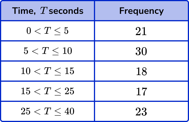
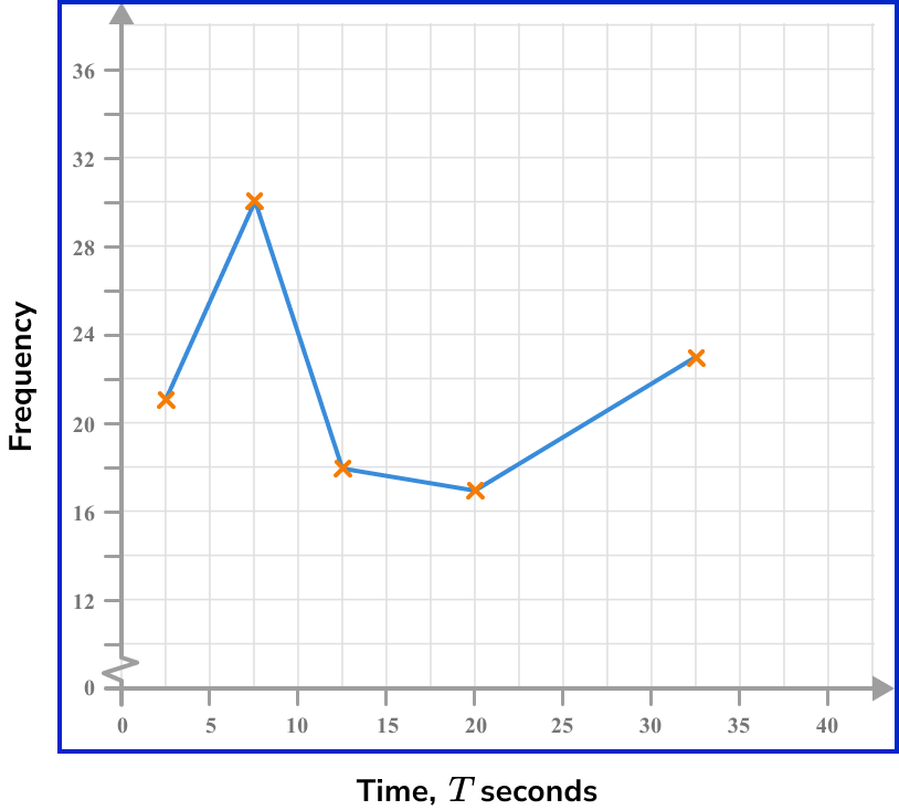
I have done a fair bit of data visualisation, but the first time I have come across "Frequency Polygons" is in a school level maths test. They are (badly) described by BBC Bitesize with is kind of the UK maths curriculum, and slightly better here but I cannot find either the rational for choosing this graph type or the exact rules, in particular with uneven bin sizes.

To show what I mean, here is some data presented as a histogram, which I think is the primary way to show this sort of data:

Following the rules of the second link, particularly "Example 6: different class intervals", the frequency polygon should look like this, as I plot counts. This seems wrong to me.

This is the equivalent barchart, which I cannot produce without an error because it is so wrong

This is a "frequency polygon" but plotting density, which seems better but still has less information than a proper histogram and no obvious advantages. It is also not what the instructions say.

For completeness this is the kernel density estimate, which is possibly better if you really want a line, but I do not like as it seems to invent features. Also no one is doing this by hand in a maths lesson at school.

Spoiler R Code to create images :

Temperature <- airquality$Temp

png("histogram.png")
hist(Temperature,breaks=c(55,60,70,75,80,100),freq = FALSE, main="Histogram")
dev.off()

png("barchart.png")
tempHist <- hist(Temperature,breaks=c(55,60,70,75,80,100),freq = TRUE, main="Bar Chart (wrong areas)")
dev.off()

png("polygonCounts.png")
plot(tempHist$mids,tempHist$counts,type="l",main="Frequency polygon with counts")
dev.off()

png("polygonFrequency.png")
plot(tempHist$mids,tempHist$density,type="l",main="Frequency polygon with density")
dev.off()

png("density.png")
plot(density(Temperature),main="Kernel density estimate")
dev.off()

 

[Kyriakos]

^Going by this link, it appears to be meant to typically divide frequencies in equal ranges and then draw them as a function (linear). The result is that this is... some 'derivative' that shows alterations in regards to how many cases there are at each midpoint?
Eg I read this example:

Slope between the midpoint 50 and midpoint 150 is 5. Can you use this to (more quickly than with other graphs) establish slope if you set a different midpoint (and if you are not a computer?)
I suppose you would be best positioned to answer this last suspicion - is there any chance that the strange method of graphing has potential benefit if you strictly work with computer programs?

 

[Samson]

^Going by this link, it appears to be meant to divide frequencies in equal ranges and then draw them as a function (typically linear). The result is that this is... some 'derivative' that shows alterations in regards to how many cases there are at each midpoint?
Eg I read this example:
View attachment 724953
Slope between the midpoint 50 and midpoint 150 is 5. Can you use this to (more quickly that with other graphs) establish slope if you set a different midpoint (and if you are not a computer?)

I was going by example 6 on that page, which uses unequal frequency ranges. The point is sometimes you are only given the bins, you cannot split them up.

 

[Kyriakos]

^My hunch would be that they mean for this to be used with some specific computer program - maybe one that kids have access to through school etc, or is supported - at which case I suppose (you are the expert on that ) it would make sense to create graphs in ways that allow for optimal use (code-dependent also). Other than that... personally I can assure you there is no such graphic method presented in Greek secondary education math books.
The main ones are the known histogram and the discus-related graph (parts of a discus/pie).

So not even a way to recursively read the graph? (if you are not in the session where it was created). That is indeed strange. Saves memory though

 

[Kyriakos]

Hm, would you say that this is a rigorous proof? (about what the vertex of a quadratic function will be, for xeR)